¹FIAB, Florence, Italy.

²Department of Mathematics and Informatics U. Dini, Univ. of Florence, Italy, Associated to IASI_CNR, Rome, Italy.2FIAB, Florence, Italy.

Corresponding Author: Antonio Fasano, FIAB SpA, via Passerini 2 50039 Vicchio (Firenze) Italy, Tel:+39 3440227030;  E-Mail: [email protected]

Received Date:   17 Oct 2018   Accepted Date:   09 Nov 2018   Published Date:  14 Nov 2018

Copyright © 2018 Fasano A

Citation: Anfuso L, Corsi M and Fasano A. (2018). Esophageal Thermal Probes: How Fast Should They Be?. Mathews J Cardiol.3(1): 018.

ABSTRACT

Background:It has been recently emphasized that the use of slow sensors to monitor the luminal esophageal temperature (LET) during atrial ablation can be seriously dangerous to the patient.

Objective:We want to investigate such a feature in a quantitative way in order to understand how fast a thermal probe should be in order to be reliable.

Methods:We formulate a model allowing reconstructing the real temperature evolution from the one recorded, knowing the sensor response time.

Results: We compare measured and real temperatures and we perform a virtual comparison among sensors with different response time starting from actual clinical data.

Conclusions:Sensors with a response time of 4 or more seconds are not safe in the presence of rapid esophageal temperature variations, i.e. when thermal monitoring is actually needed.

KEYWORDS

Atrial Fibrillation Ablation; Esophageal Temperature Monitoring; Thermal Probe Response Time; Esophageal Thermal Lesions.

INTRODUCTION

The importance of luminal esophageal temperature (LET) monitoring during procedures for pulmonary veins isolation (PVI) as a treatment of atrial fibrillation has been discussed e.g. in Kiuchi et al [1] and Koranne et al [2]. LET monitoring has been recommended in the latest expert consensus by Calkins et al [3]. In a recent paper Gianni et al [4] have reported two cases of esophageal thermal lesions (ETLs) following radiofrequency ablation (RFA) for pulmonary veins isolation (PVI), which developed to atrio-esophageal fistula (AEF), despite the detected luminal esophageal temperature (LET) had been apparently in a safe range during the whole procedure. They rightly attributed this unfortunate outcome to the large response time of the esophageal thermal probe (ETP) used, thus pointing out the great relevance of such a parameter. In the quoted paper the response time of two single sensor probes was reported (both by Smiths Medical, Dublin, Ohio, USA): the 18F esophageal stethoscope, ER400-18, and the 9F ETP ER400-9 probe, with the respective response time of 33.45s and 8.26s. Of course, the first value is so high to conceal the actual LET evolution, providing physicians with a dangerously wrong information. As remarked by Fasano [5], the second value may look OK, but it is still too large, precisely when patients are exposed to critically steep thermal gradients, i.e. when ETPs are mostly needed. The necessity of using fast sensors is stressed also by Liu et al [6] in their basic review paper. We believe that such an issue is so important that we decided to perform a quantitative analysis, trying to reconstruct the time behavior of the real temperature from the one measured by a sensor whose response time is known, with the aim of establishing how fast an ETP has to be in order to be safe. Our method will also allow making a virtual comparison among sensors with different response time, starting from clinical data detected by means of a specific probe.

METHODS

We set up a mathematical model in which τ denotes the sensor response time, θ is the measured temperature, and T is the actual temperature. The most reasonable definition of τ, also adopted by Gianni et al [4], is the following. Let θ₀ be the common value of θ and T at time t = 0 and let δ be a temperature jump applied to the sensor. Then the temperature of a sensor with response time τ evolves as follows θ(t) = θ₀ + θ[1 - exp(-t/τ)]. --------------------------------->(1)

Now, take a sequence of time instants 0, t₁ , t₂, ... , t_i, t_i+1, ... and set θ_i = θ(t_i), T_i = T(t_i). According to (1), the variation of θ in the interval (t_i, t_i+1) is (θ_i+1 - θ_i ) ~ (T_i+1 - θ_i) t_i+1 - t_i/τ,----------------------------------->(2)

provided that t_i+1 - t_i << τ . Note that (2) makes no sense if τ = 0, which entails θ = T. Taking the limit t_i+1 - t_i-> 0,we find the desired relationship: T = θ + τ dθ/dt-------------------------->(3)

Such an equation can be used for various purposes. One can enter a typical time evolution of θ and get the time course of the associate real temperature T, so to realize how large the influence of the parameter τ is. Conversely, the same equation can be used to infer the sensor response θ(t) caused by a known applied temperature T(t). Likewise, it is possible to put in (3) a sufficiently smooth interpolation θ of the clinical data of the patient’s LET in order to retrieve the real esophageal temperature T during the PVI procedure. The latter property can also be used to make a virtual comparison of ETPs with different response times. The results below will highlight the crucial role of such a parameter.

The clinical data that are going to be used were obtained at the Istituto Clinico Mediterraneo, Agropoli, Italy by Dr Giuseppe De Martino using Esotherm probe and Esotest monitor (FIAB, Italy)

RESULTS

Equation (3) illustrates very clearly that the discrepancy between measured and real temperature is nothing but the product of the sensor response time and the speed of variation of its temperature. Suppose for instance that at some instant the sensor temperature is increasing at the rate 0.25°C/s (values found in practice normally range between 0 and 1°C/s).. Then the difference T - θ is readily provided by (3) as 0.25τ, which amounts to 8.4°C and to 2.0°C for the two sensors dealt with in Gianni et al [4]. The first value is huge and it is very unlikely that such a slow sensor can react at that given rate, but the second is large too in the ablation context, since it could lead to serious lesions. One should also consider that the decision of interrupting power supply when the detected temperature goes above some selected threshold might take some seconds and that LET will anyhow increase for a while after RF has been switched off. We organize this section in three parts:

• (I) Take for θ a typical behavior of a sensor during a procedure, i.e. a temperature spike, and derive the corresponding real temperature T, knowing the sensor response time.
• (II) Take a driving temperature T (the real LET) approaching exponentially some limit T^* beyond an alarm threshold, and compute the delay with which different sensors reach the alarm temperature.
• Take clinical data recorded by means of a fast sensor and derive what the response of slower sensors would have been.

The corresponding results will emphasize the great risk of using ETPs that are not sufficiently fast.

From recorded to real LET. An easy way of seeing (3) at work is to take for θ a Gaussian curve, which is reasonably representative of a real behavior for a RFA procedure: θ(t) - θ₀ = (θ^* - θ₀ exp[ - (t - t^*)²/λ]----------------------------->(4) Here the maximum temperature θ^*represents a threshold that the operator managed not to exceed, using the information from a sensor with a given response time τ. We are going to reconstruct the real temperature T corresponding to different values of τ and of the maximum slope of θ (i.e. of the parameter λ).

We choose λ in such a way that θ has a prescribed maximal slope S, according to the formula λ = 2(θ^* - θ₀)²/eS² (see Table 1).  For not exceedingly slow sensors the three values chosen correspond to safe (0.1°C/s), alarming (0.25°C/s), critical(0.5°C/s) situations.

Table 1: Values of λ corresponding to a given maximal slope of function (4) with θ^* -θ₀ = 4°C.

S(0C/S)	0.1	0.25	0.5
λ(S2)	1177.21	188.35	47.09

The corresponding explicit expression of T is T(t) - θ₀ = (θ^* - θ₀)exp[ - (t - t^*)²/λ] {1 - 2(t - t^*)τ/λ}----------------------->(5) We can take e.g. θ₀* = 40°C(threshold measured LET). The corresponding graphs are reported in Figure 1.

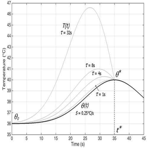
Figure 1: Behavior of the real temperature T associated to a measured temperature θ for different response times.

One more feature that can be deduced from (3) and clearly shown in Figure 1, is that when θ increases to a maximum θ^**, then T = θ at that point, and T > θ for t < t^*, meaning that T attains a maximum T^* > θ^* at some earlier instant. The situation is completely symmetric when θ decreases to a minimum. Table 2 reports the corresponding maxima of T for different pairs (S,τ).

Table 2: Maxima of function (5) for different pairs (S, τ).

τ(S)\ S(0C/S) procedures	0.1	0.25	0.5
1	40.003°C	40.02°C	40.02°C
4	40.05°C	40.3°C	41.0°C
8	40.2°C	41°C	42.7°C
32	42°C	46.6°C	54.5°C

Note: the chosen values for t cover the range of thermal probes on the market.

Response time and delay to alarm. Conversely, one can consider a temperature T(t) evolving to a dangerous range and see how a sufficiently large response time can induce a severe delay in alarming the operator, producing a dangerous situation. To do that we must integrate equation (3), where now T is the driving term and θ is the unknown: θ(t) - θ₀ = 1/τ ∫₀^t e^{-( t - η)/τ}(T(η)- θ₀)dη------------------------->(6) We consider T(t) - θ₀ = (T^* - θ₀){1 - e^{-t/ μ}}------------------------------->(7) namely a temperature raising to T^* at a speed depending on the parameter μ.  Plugging (7) into (6) we conclude that a sensor with response time μ reacts as follows: θ(t) = T^* - T^* - θ₀/1 - τ/ μ( e^{-t/ μ} - τ/μ e^-t/μ ) , if τ≠μ------------------->(8) and θ(t) = T^* - (T^* - θ₀)( 1 + t/τ) e^-t/μ , if τ = μ

It can be checked that O steadily increases to T^* irrespectively of the relative magnitude of τ and μ.

Let us choose T^* =45°C, well beyond an alarm temperature that we may reasonably set at 39°C (we still refer to a baseline temperature θ₀=39°C), and see how τ determines the delay at which θcrosses the same threshold and what is the actual value of T at the time it happens.

Table 3 shows the delay with which the alarm temperature is reached by a sensor along with the value of T at that time instant, for various values of τ and μ.

Table 3: Delay to alarm (in brackets) and actual temperature T at the alarm time instant.

τ\ μ[P]	6s [1°C/s]	10s [0.6°C/]	15s [0.4°C/]	30s [0.2°C/]
1s	39.95°C (1.4s)	39.59°C (1.04s)	39.40°C (1.03s)	39.2°C (1.02s)
4s	41.61°C (3.44s)	40.89°C (3.79s)	40.41°C (4.01s)	39.78°C (4.18s)
8s	42.73°C (5.84s)	41.90°C (6.6s)	41.29°C (7.2s)	40.41°C (8.02s)
32s	44.63°C (16.73s)	44.08°C (18.75s)	43.49°C (20.73s)	42.36°C (24.7s)

The values of µ are selected so that the speed of variation P of T when T = 39°C equals 0.2°C/s, 0.4°C/s, 0.6°C/s, 1°C/s, respectively.

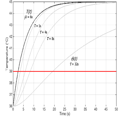
Figure 2: Sensor reaction to the driving temperature (7) for different values of τ. Here μ = 6s

Remark It is worth mentioning here that the concept of “safety threshold temperature” may be easily misunderstood, since people tend to associate it to the ideal temperature T, while it is necessarily related to the measured temperature Ɵ. Looking at Figure 2, one realizes that if it is desired that T stays below, say, 40°C, then 39°C is an appropriate threshold for sensors with τ = 1s, but for sensors with τ = 4s, τ = 8s, τ = 32s thresholds should be set at 37.2°C, 36.6°C, 36.2°C, respectively, if the baseline temperature is 36°C. Note that in the last two cases the difference between threshold and baseline temperature is close to or even less then the device accuracy, making the measure basically useless.

What can happen in practice We consider the temperature Ɵ recorded at a clinical procedure at the Istituto Clinico Mediterraneo, Agropoli, Italy (Dr Giuseppe De Martino) using a fast probe (Esotherm, FIAB, τ = 1s). We deduce the corresponding real LET T, and we derive the behavior of slower probes. We examine a case, in which RF power has been switched off at some point because the detected LET crossed the threshold and we compare the value Tc of T at that crossing time with the value T_c of T that would have been reported by slower ETPs.

Figure 3 reports the comparison between T and O for the original data (τ = 1s), and for reconstructed responses of slower ETPs (τ = 4s, τ = 8s, τ = 32s). The corresponding differences T_c -θ_c are reported in Table 4. T_c = 39.7°C

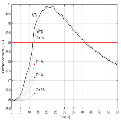
Figure 3: Temperature θ recorded with a fast probe (τ = 1s) during a clinical procedure. The dark line is the reconstructed real temperature (from eq. (3)). The three interrupted curves represent the temperatures that would have been detected by slower sensors up to the time at which θ has reached the threshold value.

Table 4: Temperature underestimation by probes with different response time.

	τ = 1s	τ = 4s	τ = 8s	τ = 32s
Tc - Ɵc (°C)	0.7	1.1	2.6	4.3

DISCUSSION

We have carried out a quantitative analysis of the influence of the response time on the behavior of a thermal sensor. While very fast sensors (response time of 1s or less) keep up rather precisely with the external stimulus, the discrepancy between the measured temperature and the real one becomes larger and larger as the response time increases. Beyond some limit, the information provided by the sensor to the operator during RFA or CA becomes so inaccurate to represent a real danger. Such a feature is more dramatic in the presence of rapid temperature variations (which are accompanied by steep thermal gradients in the area surrounding the ablator), namely in the cases where LET measurement is essential. These facts have been pointed out based on numerical simulations performed both on ideal cases and on clinical data. We have applied our method to perform a virtual comparison among different sensors, since we are able to retrieve the real LET from the one measured by means of a given sensor and in turn to predict the corresponding response of different sensors.

CONCLUSIONS

It is fairly obvious that a delayed response of a thermal sensor on an ETP will cause a delay in alarming the operator. However, for the clinical practice it is very important to translate such a simple remark into quantitative terms. The analysis here performed shows that the use of probes with response time of 4s or more must be avoided, since the information they provide is deceitful when LET varies particularly rapidly, namely precisely when LET monitoring is essential. In particuar, we have pointed out the following features, all emphasizing the danger connected to the use of slow probes:

• The real temperature T associated to a measured spike θ has a maximum exceeding the one of θ and occurring earlier. The size of such discrepancies is strongly related to the sensor response time τ
• For a given temperature T evolving beyond a given alarm temperature, the delay with which the measured temperature θ crosses the same threshold is largely increasing with the sensor response time τ.
• If RF power is switched off at some chosen temperature detected by a fast sensor, the temperature that would have been shown by a slower sensor at the same time is lower, and considerably lower if its response time τ is large.

DECLARATIONS

Competing interests Antonio Fasano is Scientific Director and R&D Manager at FIAB, Italy. Luca Anfuso and Massimo Corsi are researchers at FIAB, Italy.

ACKNOWLEDGEMENTS

We thank Dr Giuseppe De Martino allowing the use of the data recorded by him during a procedure performed at Istituto Clinico Mediterraneo, Agropoli, Italy.

REFERENCES

1. Kiuchi K, Okajima K, Shimane A, Kanda G, et al. (2016). Impact of ETM guided atrialfibrillation ablation on preventing asymptomatic excessive transmural injury. J Arrhythm. 32(1): 36-41
2. Koranne K, Basu-Ray I, Parikh V, Pollet M, et al. (2017). Esophageal Temperature Monitoring During Radiofrequency Ablation of Atrial Fibrillation: A Meta-Analysis. J A Fib. 9(4): 1452.
3. Calkins H, Hindricks G, Cappato R, Kim Y-H, et al. (2017). 2017 HRS/EHRA/ECAS/APHRS/SOLAECE expert consensus statement on catheter and surgical ablation of atrial fibrillation: Executive summary. Heart Rhythm. 14(10): e445:e494.
4. Gianni C, Atoui M, Mohanty S, Trivedi C, et al. (2016). Difference in thermodynamics between two types of esophageal temperature probes: insights from an experimental study. Heart Rhythm. 13(11): 2195-2200
5. Fasano A. (2017). To the Editor - Importance of response time of esophageal thermal probe. Heart Rhythm. 14(1): e2.
6. Liu E, Shehata M, Liu T, Amorn A, et al. (2012). Prevention of esophageal thermal injury during radiofrequency ablation for atrial fibrillation. Journal of Interventional Cardiac Electrophysiology. 35(1) : 35- 44.